Building a MLP from scratch: Torchless XOR/MNIST

To get a better understanding of how deep learning works we will have a look under the hood and implement a simple MLP from scratch (with CUDA).

Table of Contents

1. Outline
2. MLPs and gradient descent
3. Prototyping with Numpy
4. MNIST dataset and cross-entropy loss
5. Implementation in C++

Outline

In this blog post I will go through the process of building a simple MLP from scratch. The model will be applied to the XOR problem and the MNIST dataset. Since the goal of this blog post is to get a better understanding of how models work under the hood, we will not make use of any existing libraries or frameworks. Derivations for all mathematical results and the most important code snippets will be included. First, we will prototype using Numpy and then we will implement each component in C++. Lastly we will add CUDA support to speed up computations. All code can be found on GitHub.

MLPs and gradient descent

The XOR problem

The XOR problem is a problem where the task is to predict the output of the XOR operator. The XOR operator takes two binary inputs and returns one binary output. This problem is used because it is a simple non-linear problem that can be learned by a simple MLP.

Binary classification using the sigmoid function

To model the XOR function, we can create a function that takes two inputs and returns a single output in the range of $(0, 1)$. When this value is above $0.5$ we predict a $1$ and if it is below, we predict a $0$. A function that we can use to do this is the sigmoid function, which scales all values between $0$ and $1$.

$\hat{y} = \sigma(z) = \frac{1}{1 + e^{-z}}$

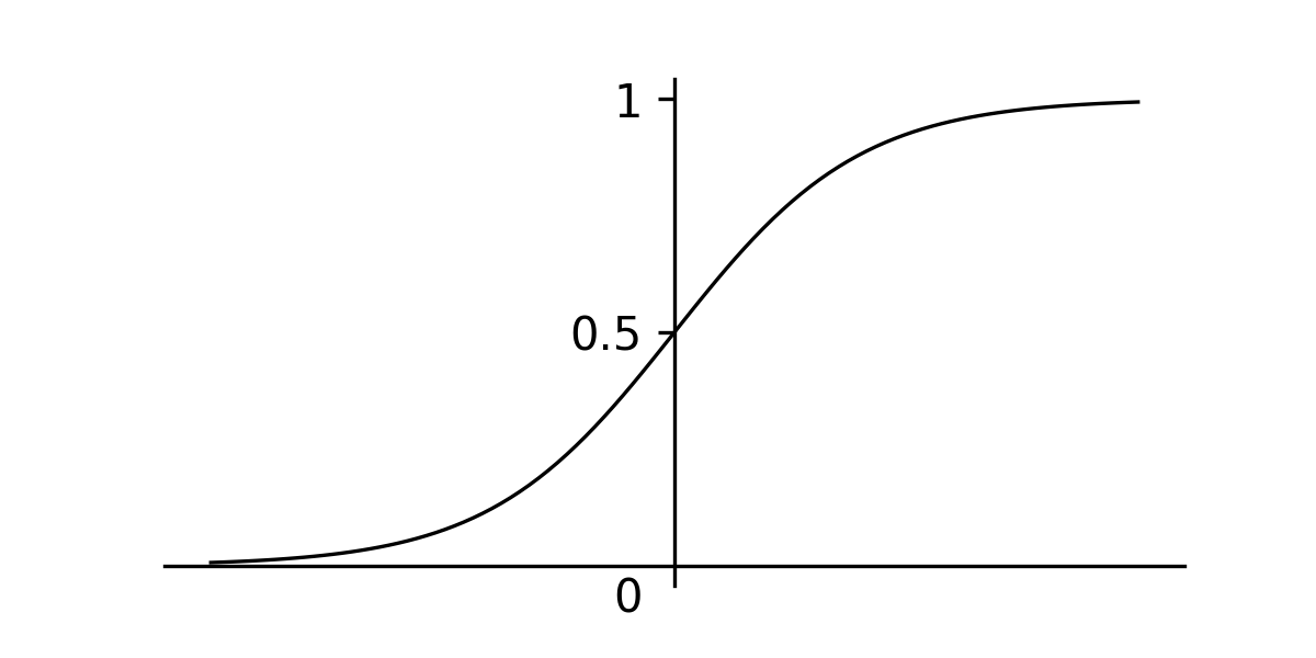
Sigmoid function

This means that the probability of a single datapoint is given by the bernoulli distribution with a probability $\hat{y_i}$: the probability of choosing $y_i = 1$ is $\hat{y_i}$ and the probability of choosing $y_i = 0$ is $1 - \hat{y_i}$.

The Multilayer Perceptron

We now know how make a prediction given a function that takes two inputs and produces a single output. How can we model this function?

One way of doing this is by using a Multilayer Perceptron (MLP). A MLP constists of two building blocks. The first creates a linear combination of the inputs and adds a bias term. The second passes the result of this linear combination through a non-linear activation function to ensure the model can learn non-linear relationships between the inputs and outputs. Each combination of weight and and bias can be seen as a neuron of the MLP. The simplest MLP we can create for this problem has two neurons.

Lets say $x_1 = 0$ and $x_2 = 1$, $w_1 = 4$ and $w_2 = -3$ and the biases are $0$. Then the model will output a prediction of $0$.

The outputs that are passed through the activation functions can be passed on to the next layer of the MLP and so on. This can be visulized as a graph where the each edge represents a weight, the nodes make a linear combinations of the resulting values and add a bias term.

Graph visualization of a MLP

Passing the input through the layers of an MLP is often referred to as forward propagation or a forward pass. It is important to note that any non-linear activation function can be chosen instead of the sigmoid function. In practice many different functions are used, each having their own advantages and disadvantages. In this section we have fully written out the matrices for the fully connected layer in an MLP. However usually we will write such computations in matrix form. The matrix for representation of the first fully connected layer visualized above is given by the following equation.

However, for convience we will transpose the features and labels so they can be staked in a large matrix $\mathbf{X}$ and $\mathbf{Y}$. This will also make the gradients align better with the shapes of the weights and biases.

Maximum likelihood estimation

To optmize the parameters of the MLP, we want to find the values of the weights and biases that best explain the data. This is process is called maximum likelihood estimation (MLE). The probability of the data given the parameters can be expressed as the product of the probabilities of each data point given the parameters assuming that each data point is independent of the others and is drawn from the same distribution (this assumption is referred to as independently and identically distributed, or i.i.d. for short). It is important to understand that the likelihood function is a function of the parameters and not the data. This means the likelihood function is not a probability distribution and is therefore also referred to as a function.

Instead of maximizing the likelihood function, we usually minimize a the negative log-likelihood which is an equivalent problem and allows us to formulate the problem in terms of a loss that we can minimize. Maximizing the likelihood function is equivalent to maximizing the log-likelihood function because the log is a monotonically increasing function.

Using the rules for logarithms, this can be simplified resulting in the binary cross-entropy loss. Later we will derive a more general formulation of this loss function that can be for classification problems with many classes called the cross-entropy loss.

Multivariate calculus, the chain rule and Jacobians

Before we do this, we should give a brief introduction to multivariate calculus and how the chain rule can be used to compute derivatives. In multivariate calculus, each function has multiple inputs and outputs and so we can compute partial derivatives for each output with respect to a specific input. When we do this, we treat all other inputs and outputs as constants.

A Jacobian is a matrix that contains the derivatives of a multi-variate function with respect to each parameter. The element in the $i$-th row and $j$-th column of the Jacobian is the derivative of the $i$-th output with respect to the $j$-th input. One example is given above, lets look at one more example.

Now lets derive the derivative of a dot product with respect to the inputs. To do this we first compute the partial derivative with respect to one input $x_i$. Then we can replace the derivative with the kronecker delta wich is only one if $i = j$ and zero otherwise, this is true because only that term has an effect for the derivative of $x_i$ all other terms are treated as constants. The kronecker delta then cancles out the sum and we can replace all subscripts $i$ with $j$. Since this function has one output the final results will be $\in \mathbb{R}^{1 \times N}$. based on the derivative of one element we can conclude that the full derivative is $\mathbf{w}^{\top}$.

Lastly we need to understand how the chain rule can be used to compute derivatives of nested functions. The full MLP is a composition of multiple functions and if we understand how derivatives propagate over compositions of functions, we can compute the derivatives of the loss with respect to each parameter of the MLP.

The chain rule states that the derivative of a composition of functions is the derivative of the outer function evaluated at the inner function, multiplied by the derivative of the inner function. Since the model contains many parameters, we compute partial derivatives, treating all parameters except one as constants.

Lets look two examples of how the chain rule can be applied.

When computing derivatives it is important to think about how each parameter influences the gradient. There can be multiple paths when a variable occurs multiple times in one function and all these seperate paths need to be added together. Below is an example of this.

Gradient descent and gradients for binary cross-entropy

To find the optimal parameters of this function we need to find the place where this loss function is minimal. At this location, the derivative of this function is zero, so the full analytical solution can be derived by taking the derivative of the function and setting it to zero. However, often this is not feasible for larger datasets and complex models. Instead, we can therefore use an optimization algorithm called gradient descent. The idea behind this algorithm is that we can iteratively take small steps in the opposite direction of the gradient to find minimum of the function. To understand why this works, we need to understand what the gradient means. If we compute the gradient of the function w.r.t a specific parameter, that gradient tells us the direction of steepest ascent when changing that specific parameter. By iteratively taking small steps in the opposite direction of the gradient simultaneously for each parameters we can find the minimum of the function (if the function is convex).

Lets use the chain rule to compute the derivative of the loss function with respect to the weights and biases. We start by computing the derivative of the loss function for one output with respect to its inputs. Note that we can remove the summation here because all components of the summutation of indixes $i \neq j$ are $0$.

So the derivative of the loss function here is a vector of size $n$ where each element is the derivative of the loss function with respect to the $i$-th input. Next we can compute the derivative of the sigmoid function with respect to its input. Since we know that $\hat{y_j} = \sigma(z)$, and $\frac{\partial}{\partial z} \sigma(z) = \sigma(z)(1 - \sigma(z))$, we can compute the derivative of the sigmoid function with respect to its input.

This can then be used to compute the derivative of the loss function with respect to the input of each activation using the chain rule, the differences between the actual labels and the predicted labels.

The full Jacobian will then be a vector $\in \mathbb{R}^{1 \times N}$ with the differences between the probabilities and the actual labels.

Derivatives of the fully connected layer

Recall that we can write the linear combination of the inputs and biases an matrix form.

Lets compute the gradient of this equation with respect to the weights $\mathbf{W}$ and biases $\mathbf{b}$ and the inputs $\mathbf{x}$.

Assuming that the number of input nodes are $M$ and the number of output nodes are $N$, the Jacobian will be an identity matrix $\in \mathbb{R}^{N \times M}$.

To find the gradients of the bias we with respect to the loss, we can the multiply the Jacobian of loss w.r.t the activations with the gradient we just found. This means mutliplying a matrix $\in \mathbb{R}^{1 \times N}$ with a matrix $\in \mathbb{R}^{N \times M}$ to get a matrix $\in \mathbb{R}^{1 \times M}$ which has exactly the same shape as the bias. The gradient of the bias thus essentially sums over the gradients of the loss with respect to the activations.

Next, let’s compute the gradient of the loss with respect to the inputs $\mathbf{x}_i$, which can be passed on to the next layer of the MLP to compute the gradients for that layer. Just like with the bias, we will look at the gradient for one specific element in $\mathbf{y}_i$ with respect to one specific element in $\mathbf{x}_i$. Which results in the matrix $\mathbf{W}^\top$ which can be mutliplied again with the gradients with respect to the activations to find the full derivative with respect to the loss. The resulting vector will be $\in \mathbb{R}^{1 \times M}$.

Lastly we will compute the gradient of the loss with respect to the weights $\mathbf{W}$. This is a bit more complex than the previous cases. Therefore we look at the derivative of the output with respect to one element in the weight matrix $\mathbf{W}$. That gradient will be a vector, which means that the full Jacobian will be a matrix with $4$ dimensions, however this simplifies when multiplied by the gradients of the activations.

Now we can multiply this with the gradients of the activations to get the full gradient with respect to the weights. The resulting matrix will be $\in \mathbb{R}^{M \times N}$.

This means that the overall gradient can be written as the outer product between the features of the $i$-th data point and the gradients of the loss w.r.t the activations.

Backpropagation and stochastic gradient descent

We have now computed all gradients needed to optimize the parameters of the model. The method we used for computing the gradients is called backpropagation, because we start with the gradients of the loss functions and propagate them backwards through the model until we reach the input of the model. After computing all gradients the next step is to use these gradients to update the parameters of the model.

As we discussed earlier, this can be done by updating each parameter in the opposite direction of the gradient. The size of the steps we take is referred to as the learning rate. The learning rate is a hyperparameter that we can tune to our problem. If our steps are too large, the model will overshoot the minimum of the loss function and if our steps are too small, the model will take too long to converge.

Usually the gradient is not computed for the entire dataset, but for a subset of the data referred to as a mini-batch. The gradient of the mini-batch then gives us an approximation of the gradients of the entire dataset. The mini-batches are randomly selected from the dataset and the stochastic nature of the procedure can help to avoid local minima in the loss function. This variation of the gradient descent algorithm is therefore referred to as stochastic gradient descent (SGD).

In the next section we will build a prototype of the model using Numpy in Python.

Prototyping with Numpy

First we need to create a dataloader that can be used to generate batches of data samples. We will do this by sampeling from a uniform distribution and setting values to $0$ or $1$ with a probability of $0.5$. We then create the labels by applying the XOR operation to the samples. We implement the dataloader using the __next__ dunder method, which allows us to iterate over the generated batches. We pass along the random generator so we can set one seed and make results reproducible. A bit of noise is added to the data to make the problem a bit more interesting and it will enable us to visualize the decision boundaries.

# src/dataloaders.py

class XORDataLoader:

    def __init__(self, batch_size: int, noise_std: float, rng: np.random.Generator):
        self.batch_size = batch_size
        self.noise_std = noise_std
        self.rng = rng

    def __next__(self):
        a = self.rng.integers(0, 2, size=(self.batch_size,))
        b = self.rng.integers(0, 2, size=(self.batch_size,))

        y = a^b
        x = np.stack((a, b), axis=1)
        noise = self.rng.uniform(0, self.noise_std, size=x.shape)

        return x + noise, y

Next, we will implement an abtract base class for the modules of our MLP. For each module we will implement four different methods. The forward method computes the output of the module given the input. The backward method computes the gradients of the loss w.r.t the output of the module. The update method updates the weights for that module using the given learning rate. The zero_grad method resets the gradients to zero for this module.

# src/modules.py

class Module(ABC):
    """Base class for all neural network modules"""

    @abstractmethod
    def forward(self, x) -> np.ndarray:
        """Forward pass for this module (compute the output)"""
        pass

    @abstractmethod
    def backward(self, grads) -> np.ndarray:
        """Backward pass for this module (compute the gradients)"""
        pass

    @abstractmethod
    def update(self, learning_rate: float):
        """Update the weights of this module"""
        pass

    @abstractmethod
    def zero_grad(self):
        """Reset the gradients of this module"""
        pass

We are now ready to implement the fully connected layer. Here we use the numpy broadcasting features to vectorize the computation over the entire batch. The grads parameter of the backward gives us the gradients of the loss w.r.t to the outputs of this module. We can then compute the gradients for the weights of this module using the rules we derived in the previous section. Note that we take the average of the gradients over the entire batch. Additionally we can cache computations for the forward pass to avoid recomputing the same values during backpropagation.

Xavier initialization is a popular choice for initializing the weights of a neural network. It is an initialization technique that ensure that the gradients of the weights are approximately the same for all layers in the network. Maybe I will do a more detailed explanation of this in a future blog post.

# src/modules.py

# ...

class LinearLayer(Module):

    def __init__(self, in_features, out_features, rng: np.random.Generator):
        self.in_features = in_features
        self.out_features = out_features

        limit = np.sqrt(6 / (in_features + out_features))
        self.w = rng.uniform(-limit, limit, size=(out_features, in_features))
        self.w_grads = np.zeros_like(self.w)

        self.b = np.zeros((out_features,))
        self.b_grads = np.zeros_like(self.b)

    def forward(self, x):
        self.cached_input = x
        return x @ self.w.T + self.b

    def backward(self, grads):
        self.b_grads = grads.sum(axis=0) / grads.shape[0]
        self.w_grads = grads.T @ self.cached_input / grads.shape[0]
        return grads @ self.w

    def update(self, learning_rate: float):
        self.w -= learning_rate * self.w_grads
        self.b -= learning_rate * self.b_grads

    def zero_grad(self):
        self.w_grads = np.zeros_like(self.w)
        self.b_grads = np.zeros_like(self.b)

Next, we will implement a module for the activation functions that we use in our MLP. For the XOR problem we will make use of the tanh function. Since this function does not have any parameters itself, we only need to compute the gradients with respect to the inputs of this function.

# src/modules.py

# ...

class Tanh(Module):
    """Tanh activation function"""

    def forward(self, x):
        self.cached = np.tanh(x)
        return self.cached

    def backward(self, grads):
        return grads * (1 - self.cached**2)

    # ...

That gives us all the components we need to implement our MLP. The forward pass will compute the output of the MLP given the input. The backward pass will compute the gradients of the loss w.r.t the output of the MLP and the gradients of each of the layers. The update method will update the weights of the MLP using the given learning rate. The zero_grad method will reset the gradients to zero for each layer in the MLP.

# src/modules.py

# ...

class MLP(Module):
    """Multi-layer perceptron"""

    def __init__(
        self,
        in_features: int,
        hidden_features: int,
        out_features: int,
        rng: np.random.Generator,
        activation: Module = Tanh(),
    ):
        self.layers = [
            LinearLayer(in_features=in_features, out_features=hidden_features, rng=rng),
            activation,
            LinearLayer(in_features=hidden_features, out_features=out_features, rng=rng),
        ]

    def forward(self, x):
        for layer in self.layers:
            x = layer.forward(x)
        return x

    def backward(self, grads):
        for layer in self.layers[::-1]:
            grads = layer.backward(grads)
        return grads

    def update(self, learning_rate: float):
        for layer in self.layers:
            layer.update(learning_rate)

    def zero_grad(self):
        for layer in self.layers:
            layer.zero_grad()

Now we can implement the loss function (binary cross-entropy) and its gradient. We use the derivatives we derived in the previous section. Note that we clip the probabilities to prevent the probabilities being exactly 0 or 1, which would cause the log to be undefined.

# src/losses.py

def binary_cross_entropy_loss(
  probs: np.ndarray,
  labels: np.ndarray,
) -> Tuple[np.float64, np.ndarray]:
    probs = np.clip(probs, 1e-7, 1 - 1e-7)
    labels = labels[:, np.newaxis]
    loss = -(labels * np.log(probs) + (1 - labels) * np.log(1 - probs)).mean()
    grads = probs - labels
    return loss, grads

Finally we can write the training loop for the MLP. For this problem the following parameters will lead to convergence, sometimes faster, sometimes a bit slower depending on the seed. The code can be run using the command python3 -m src.xor. We have added a stopping condition that will stop training if the loss has not changed enough. Feel free to play around with the parameters, number of nodes/layers, etc.

# src/xor.py

noise_std = 0.1
num_epochs = 1000
batches_per_epoch = 10
batch_size = 64
lr = 0.05
rng = default_rng(seed=42)

dl = XORDataLoader(batch_size, noise_std, rng)
model = MLP(in_features=2, hidden_features=4, out_features=1, rng=rng)

losses = []
accs = []

for epoch in range(num_epochs):
    avg_loss = 0
    avg_acc = 0

    for _ in range(batches_per_epoch):
        x, y = next(dl)
        logits = model.forward(x)

        probs = sigmoid(logits)
        preds = (probs >= 0.5).astype(int)
        acc = ((preds.squeeze() == y).sum() / batch_size).item()

        loss, grads = binary_cross_entropy_loss(probs, y)

        model.backward(grads)
        model.update(learning_rate=lr)
        model.zero_grad()

        avg_loss += loss.item()
        avg_acc += acc

    avg_loss /= batches_per_epoch
    avg_acc /= batches_per_epoch

    losses.append(avg_loss)
    accs.append(avg_acc)

    print(f"Epoch {epoch} {avg_acc=} {avg_loss=}")

    if epoch > 0 and abs(losses[-1] - losses[-2]) < 1e-5:
        break

To see how the model learns, we can plot the losses and accuracies over epochs. Its clear that the model already has a high accuracy before the loss converges, and this is because it has to be absolutely certain in its predictions to minimize the loss function. Additionally, Since the XOR problem is a relatively simple problem with just two inputs, we can get a feeling for our models decision boundaries by plotting labels for various inputs.

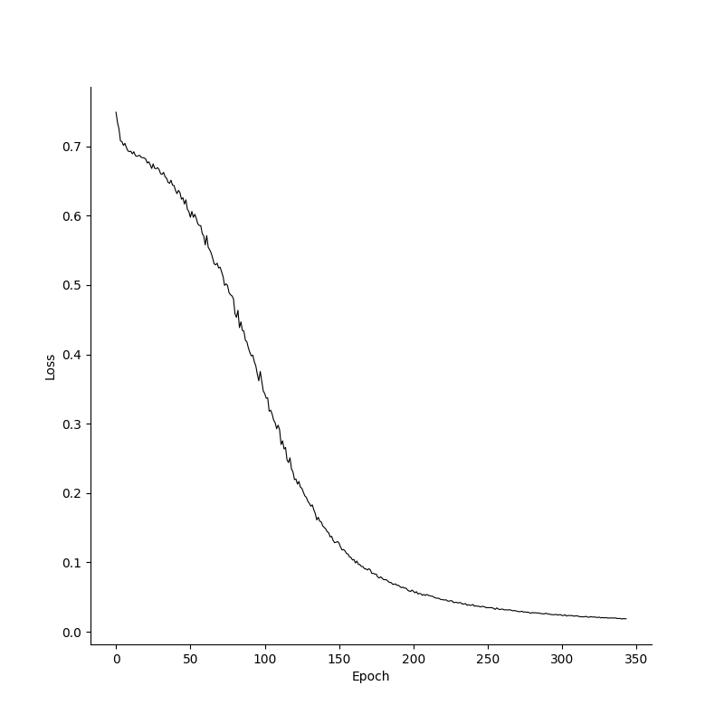
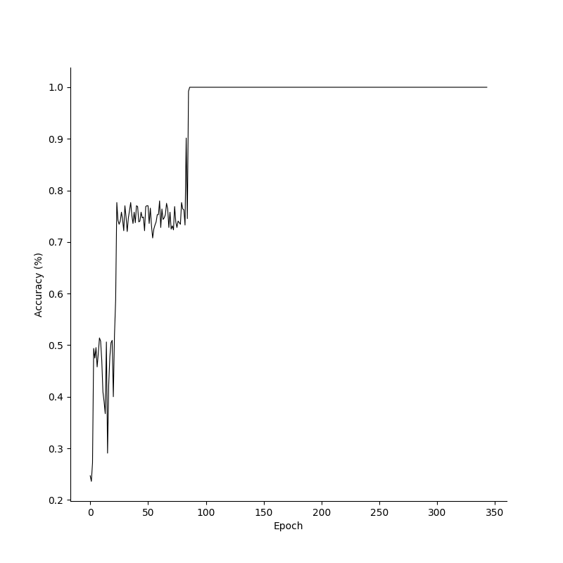
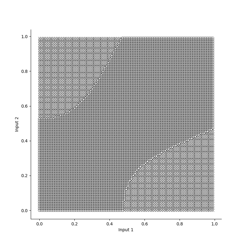
Losses, accuracies and decision boundaries for the XOR prototype in Numpy

MNIST dataset and cross-entropy loss

For a problem such as the XOR problem we do not need many nodes in our MLP, and so the speed of operations is not a problem. However, for more complex problems , where we have a large number of nodes, the speed of operations does become a problem. Here we will see a noticable increase in speed once we add GPU support. Application to the MNIST dataset is relatively straightforward, however we will need to define a dataloader for the dataset and derive and implement the cross-entropy loss function which will allow us to classify multiple classes instead of just two.

MNIST dataset

The MNIST dataset is a dataset of handwritten digits from zero to nine. It consists of 60,000 images of size 28x28 pixels. Each image is a grayscale image with a single digit. The dataset is divided into a training set and a test set. The training set contains 50,000 images and the test set contains 10,000 images. The images are stored in a binary file format. The dataset can be downloaded from Kaggle. If you are following along, my codebase assumes the code is placed in the mnist folder. Code for implementing the dataloader for this dataset can be found here.

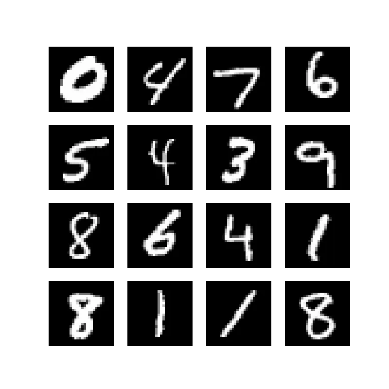
16 samples from the MNIST dataset

Cross-entropy

To encode labels for mutliple class classification we use one-hot encoding. To encode a label we create a vector of size $M$ where each element is either $0$ or $1$. If the $m$-th element is $1$, then the correct class for that label is the $m$-th class. The prediction is then one value for each class, namely the probability of that class. The probability of the correct label is then computed as follows.

Again, we can use this to compute the negative log-likelihood for the full dataset. The resulting loss is referred to as the cross entropy loss. If we think about what this log curve looks like we can see that this function is maximized when the predicted probability for the correct label is 1. The lower the probability for the correct label the higher the loss.

Before deriving the derivative we need to understand how we can ensure that the final logits are true probabilities using the softmax function. The softmax function takes a vector of size $M$ and returns a vector of size $M$ where each element is the probability of that class. The softmax function is defined as follows.

By dividing by the sum of $e$ raised to the power of each element, we ensure that the if we sum all resulting values they sum up to $1$. Because we are taking the exponential of the elements, the resulting values are always positive.

During training it is beneficial to use the log-sum-exp trick which increases numerical stability by combining the cross entropy loss and the softmax functions. We will derive this for a single datapoint.

Now we are ready to derive the derivative of the cross-entropy loss combined with the softmax function.

Let’s implement this using Numpy.

# src/losses.py

# ...

def cross_entropy_loss(logits, labels) -> Tuple[np.float64, np.ndarray]:
    one_hot = np.zeros_like(logits)
    one_hot[np.arange(logits.shape[0]), labels] = 1

    m = logits.max(axis=-1, keepdims=True)
    exp_shifted = np.exp(logits - m)
    log_sum_exp = np.log(exp_shifted.sum(axis=-1))
    loss = np.mean(-np.sum(one_hot * logits, axis=-1) + m.squeeze() + log_sum_exp)

    softmax = exp_shifted / np.sum(exp_shifted, axis=-1, keepdims=True)
    grads = softmax - one_hot

    return loss, grads

Lastly, we can write the training loop for the MLP as before. You can try implementing this yourself (code can be found here). The tanh activation problem will work for this problem, however I suggesting experimenting with the ReLU activation function, which is defined as follows.

$\text{ReLU}(x) = \max(0, x)$

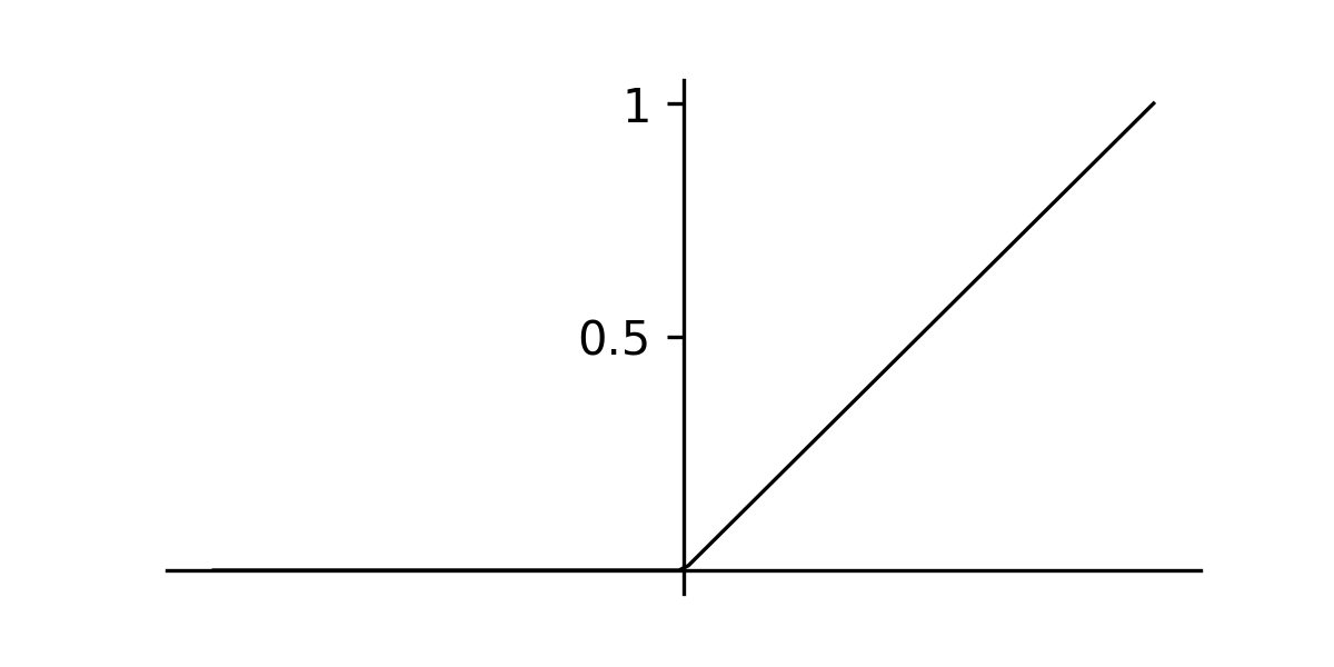
Rectified linear unit (ReLU)

With sufficient hidden neurons, the model should be able to achieve accuracy of at least $98\%$ on the test dataset. Interestingly, even with very few neurons we can achieve a suprisingly high accuracy. If you don’t get such results out of the box, try varying the batch size, learning rate, etc.

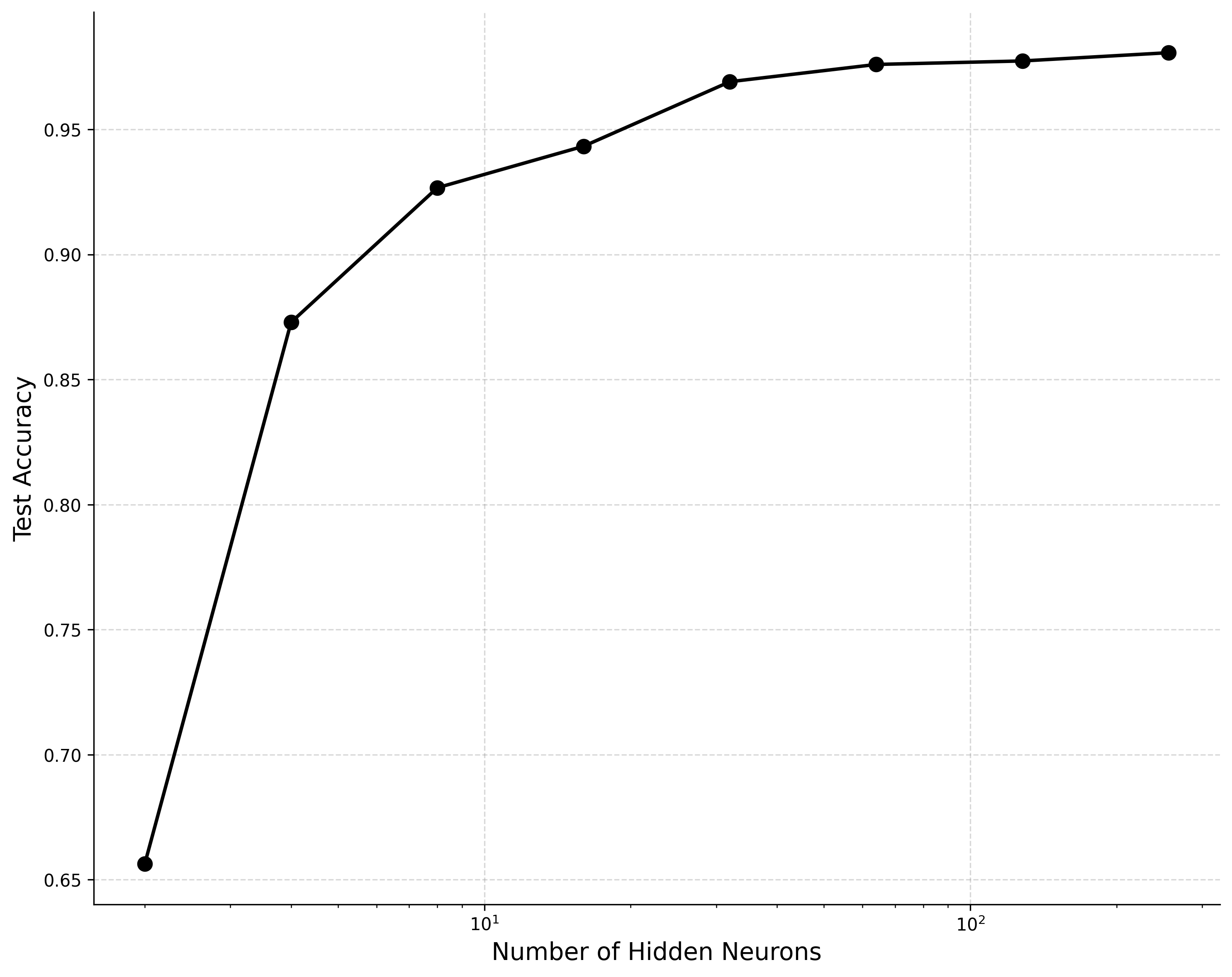
Network accuracy vs capacity on MNIST

Lastly, it can be interesting to visualize what it is that our model looks at. We can visualize this plotting the weights of our initial layer as images. If we then keep track when these neurons activate we can see what neurons are most important for recognizing a specific class of digits.

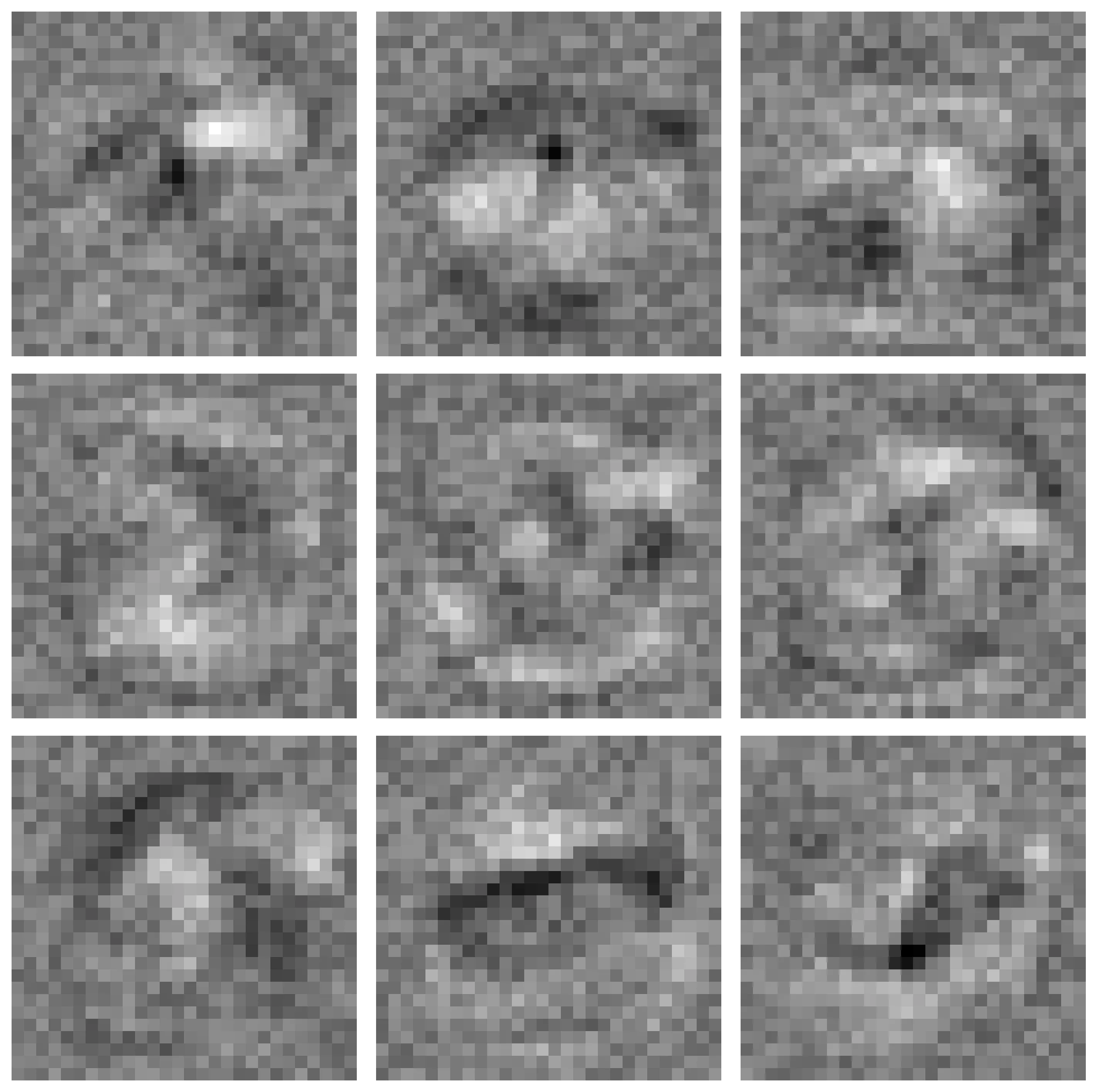
First-layer weights for an MLP with 10 hidden neurons

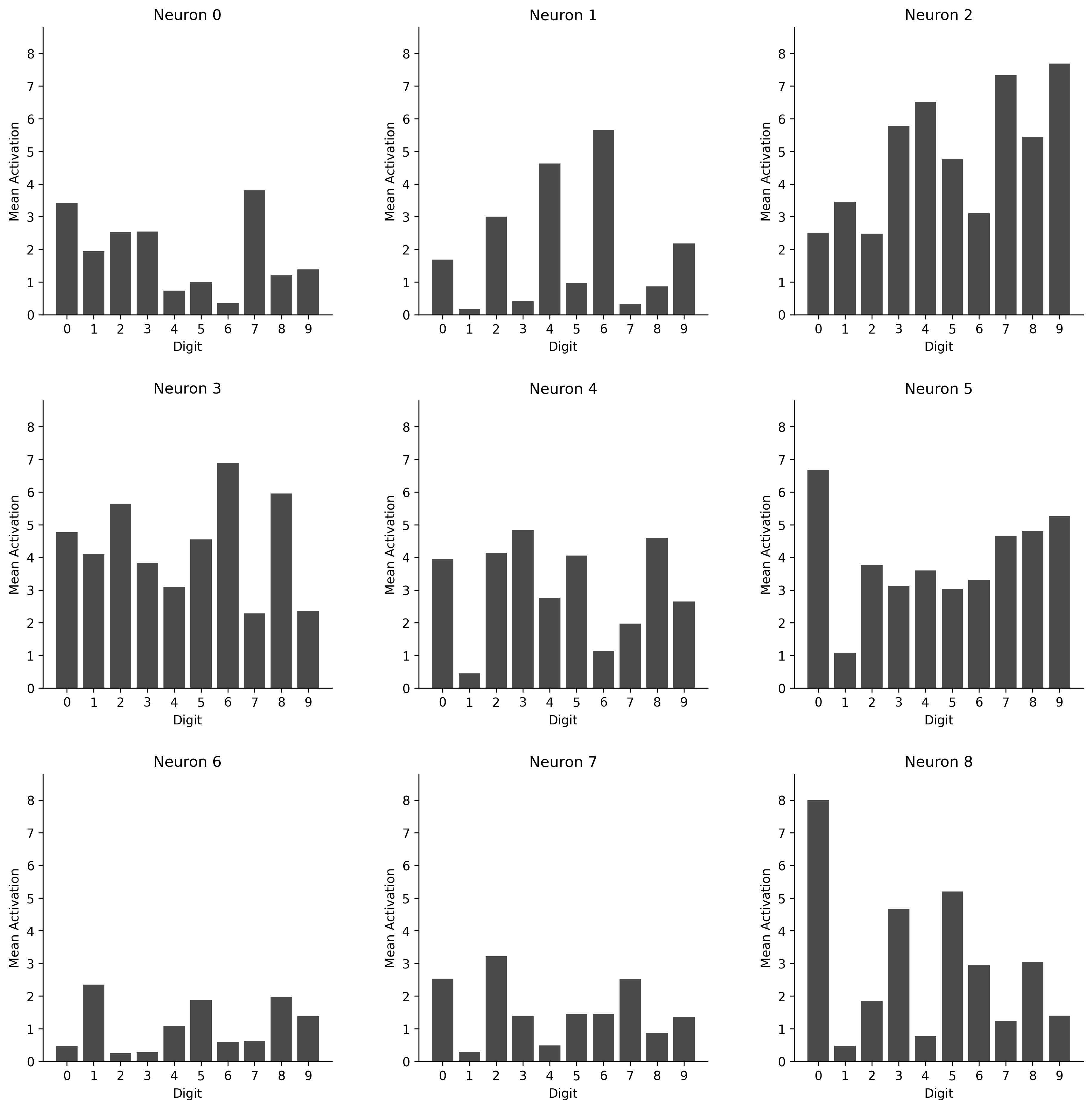
Mean activations for each input for each neuron

Implementation in C++

We are now ready to implement our models in c++ with CUDA to see if we can speed up training using a GPU.